 com.imsl.stat.ContingencyTable
|
JMSLTM Numerical Library 4.0 | ||||||||
| PREV CLASS NEXT CLASS | FRAMES NO FRAMES | ||||||||
| SUMMARY: NESTED | FIELD | CONSTR | METHOD | DETAIL: FIELD | CONSTR | METHOD | ||||||||
java.lang.Object
Performs a chi-squared analysis of a two-way contingency table.
Class ContingencyTable computes statistics associated with
an ![]() contingency table. The function computes
the chi-squared test of independence, expected values, contributions to
chi-squared, row and column marginal totals, some measures of association,
correlation, prediction, uncertainty, the McNemar test for symmetry, a test
for linear trend, the odds and the log odds ratio, and the kappa statistic
(if the appropriate optional arguments are selected).
contingency table. The function computes
the chi-squared test of independence, expected values, contributions to
chi-squared, row and column marginal totals, some measures of association,
correlation, prediction, uncertainty, the McNemar test for symmetry, a test
for linear trend, the odds and the log odds ratio, and the kappa statistic
(if the appropriate optional arguments are selected).
Notation
Let ![]() denote the observed cell frequency in the
ij cell of the table and n denote the total count in the
table. Let
denote the observed cell frequency in the
ij cell of the table and n denote the total count in the
table. Let ![]() denote the
predicted cell probabilities under the null hypothesis of independence,
where
denote the
predicted cell probabilities under the null hypothesis of independence,
where ![]() and
and ![]() are the row and column marginal relative frequencies. Next, compute the
expected cell counts as
are the row and column marginal relative frequencies. Next, compute the
expected cell counts as ![]() .
.
Also required in the following are ![]() and
and
![]() for
for ![]() .
Let
.
Let ![]() denote the row and column response of
observation s. Then,
denote the row and column response of
observation s. Then, ![]() , or
-1, depending on whether
, or
-1, depending on whether
![]() , or
, or ![]() ,
respectively. The
,
respectively. The ![]() are similarly defined in terms
of the
are similarly defined in terms
of the ![]() variables.
variables.
Chi-squared Statistic
For each cell in the table, the contribution to ![]() is given as
is given as ![]() . The Pearson
chi-squared statistic (denoted
. The Pearson
chi-squared statistic (denoted ![]() ) is computed as
the sum of the cell contributions to chi-squared. It has
(r - 1) (c - 1) degrees of freedom and tests the null
hypothesis of independence, i.e.,
) is computed as
the sum of the cell contributions to chi-squared. It has
(r - 1) (c - 1) degrees of freedom and tests the null
hypothesis of independence, i.e.,
![]() . The null
hypothesis is rejected if the computed value of
. The null
hypothesis is rejected if the computed value of ![]() is too large.
is too large.
The maximum likelihood equivalent of ![]() is computed as follows:
is computed as follows:
![]()
![]() is asymptotically equivalent to
is asymptotically equivalent to
![]() and tests the same hypothesis with the same
degrees of freedom.
and tests the same hypothesis with the same
degrees of freedom.
Measures Related to Chi-squared (Phi, Contingency Coefficient, and Cramer's V)
There are three measures related to chi-squared that do not depend on sample size:
![]()
![]()
![]()
Since these statistics do not depend on sample size and are large when
the hypothesis of independence is rejected, they can be thought of as
measures of association and can be compared across tables with different
sized samples. While both P and V have a range between 0.0
and 1.0, the upper bound of P is actually somewhat less than 1.0 for
any given table (see Kendall and Stuart 1979, p. 587). The significance of
all three statistics is the same as that of the ![]() statistic, return value from the
statistic, return value from the getChiSquared method.
The distribution of the ![]() statistic in finite
samples approximates a chi-squared distribution. To compute the exact mean
and standard deviation of the
statistic in finite
samples approximates a chi-squared distribution. To compute the exact mean
and standard deviation of the ![]() statistic,
Haldane (1939) uses the multinomial distribution with fixed table marginals.
The exact mean and standard deviation generally differ little from the mean
and standard deviation of the associated chi-squared distribution.
statistic,
Haldane (1939) uses the multinomial distribution with fixed table marginals.
The exact mean and standard deviation generally differ little from the mean
and standard deviation of the associated chi-squared distribution.
Standard Errors and p-values for Some Measures of Association
In Columns 1 through 4 of statistics, estimated standard errors and
asymptotic p-values are reported. Estimates of the standard errors
are computed in two ways. The first estimate, in Column 1 of the return
matrix from the getStatistics method, is asymptotically valid for
any value of the statistic. The second estimate, in Column 2 of the array,
is only correct under the null hypothesis of no association. The
z-scores in Column 3 of statistics are computed using this second
estimate of the standard errors. The p-values in Column 4 are
computed from this z-score. See Brown and Benedetti (1977) for a
discussion and formulas for the standard errors in Column 2.
Measures of Association for Ranked Rows and Columns
The measures of association, ![]() , P, and
V, do not require any ordering of the row and column categories.
Class
, P, and
V, do not require any ordering of the row and column categories.
Class ContingencyTable also computes several measures of
association for tables in which the rows and column categories correspond
to ranked observations. Two of these tests, the product-moment correlation
and the Spearman correlation, are correlation coefficients computed using
assigned scores for the row and column categories. The cell indices are used
for the product-moment correlation, while the average of the tied ranks of
the row and column marginals is used for the Spearman rank correlation.
Other scores are possible.
Gamma, Kendall's ![]() , Stuart's
, Stuart's
![]() , and Somers' D are measures of
association that are computed like a correlation coefficient in the
numerator. In all these measures, the numerator is computed as the
"covariance" between the
, and Somers' D are measures of
association that are computed like a correlation coefficient in the
numerator. In all these measures, the numerator is computed as the
"covariance" between the ![]() variables and
variables and
![]() variables defined above, i.e., as follows:
variables defined above, i.e., as follows:
![]()
Recall that ![]() and
and ![]() can take values -1, 0, or 1. Since the product
can take values -1, 0, or 1. Since the product
![]() only if
only if ![]() and
and
![]() are both 1 or are both -1, it is easy to show that
this "covariance" is twice the total number of agreements minus the number
of disagreements, where a disagreement occurs when
are both 1 or are both -1, it is easy to show that
this "covariance" is twice the total number of agreements minus the number
of disagreements, where a disagreement occurs when
![]() .
.
Kendall's ![]() is computed as the correlation
between the
is computed as the correlation
between the ![]() variables and the
variables and the
![]() variables (see Kendall and Stuart 1979, p. 593).
In a rectangular table
variables (see Kendall and Stuart 1979, p. 593).
In a rectangular table ![]() , Kendall's
, Kendall's
![]() cannot be 1.0 (if all marginal totals are
positive). For this reason, Stuart suggested a modification to the
denominator of
cannot be 1.0 (if all marginal totals are
positive). For this reason, Stuart suggested a modification to the
denominator of ![]() in which the denominator becomes
the largest possible value of the "covariance." This maximizing value is
approximately
in which the denominator becomes
the largest possible value of the "covariance." This maximizing value is
approximately ![]() , where
m = min (r, c). Stuart's
, where
m = min (r, c). Stuart's ![]() uses this approximate value in its denominator. For large
uses this approximate value in its denominator. For large
![]() .
.
Gamma can be motivated in a slightly different manner. Because the
"covariance" of the ![]() variables and the
variables and the
![]() variables can be thought of as twice the number
of agreements minus the disagreements, 2(A - D), where
A is the number of agreements and D is the number of
disagreements, Gamma is motivated as the probability of agreement minus the
probability of disagreement, given that either agreement or disagreement
occurred. This is shown as
variables can be thought of as twice the number
of agreements minus the disagreements, 2(A - D), where
A is the number of agreements and D is the number of
disagreements, Gamma is motivated as the probability of agreement minus the
probability of disagreement, given that either agreement or disagreement
occurred. This is shown as ![]() .
.
Two definitions of Somers' D are possible, one for rows and a
second for columns. Somers' D for rows can be thought of as the
regression coefficient for predicting ![]() from
from
![]() . Moreover, Somer's D for rows is the
probability of agreement minus the probability of disagreement, given that
the column variable,
. Moreover, Somer's D for rows is the
probability of agreement minus the probability of disagreement, given that
the column variable, ![]() , is not 0. Somers' D
for columns is defined in a similar manner.
, is not 0. Somers' D
for columns is defined in a similar manner.
A discussion of all of the measures of association in this section can be found in Kendall and Stuart (1979, p. 592).
Measures of Prediction and Uncertainty
Optimal Prediction Coefficients: The measures in this section do not require any ordering of the row or column variables. They are based entirely upon probabilities. Most are discussed in Bishop et al. (1975, p. 385).
Consider predicting (or classifying) the column for a given row in the table. Under the null hypothesis of independence, choose the column with the highest column marginal probability for all rows. In this case, the probability of misclassification for any row is 1 minus this marginal probability. If independence is not assumed within each row, choose the column with the highest row conditional probability. The probability of misclassification for the row becomes 1 minus this conditional probability.
Define the optimal prediction coefficient
![]() for predicting columns from
rows as the proportion of the probability of misclassification that is
eliminated because the random variables are not independent. It is
estimated by
for predicting columns from
rows as the proportion of the probability of misclassification that is
eliminated because the random variables are not independent. It is
estimated by
![]()
where m is the index of the maximum estimated probability in the
row ![]() or row margin
or row margin
![]() . A similar coefficient is defined for
predicting the rows from the columns. The symmetric version of the optimal
prediction
. A similar coefficient is defined for
predicting the rows from the columns. The symmetric version of the optimal
prediction ![]() is obtained by summing the
numerators and denominators of
is obtained by summing the
numerators and denominators of ![]() and
and
![]() then dividing. Standard errors for
these coefficients are given in Bishop et al. (1975, p. 388).
then dividing. Standard errors for
these coefficients are given in Bishop et al. (1975, p. 388).
A problem with the optimal prediction coefficients
![]() is that they vary with the marginal
probabilities. One way to correct this is to use row conditional
probabilities. The optimal prediction
is that they vary with the marginal
probabilities. One way to correct this is to use row conditional
probabilities. The optimal prediction ![]() coefficients are defined as the corresponding
coefficients are defined as the corresponding ![]() coefficients in which first the row (or column) marginals are adjusted to
the same number of observations. This yields
coefficients in which first the row (or column) marginals are adjusted to
the same number of observations. This yields
![]()
where i indexes the rows, j indexes the columns, and
![]() is the (estimated) probability of column
j given row i.
is the (estimated) probability of column
j given row i.
![]()
is similarly defined.
Goodman and Kruskal ![]() : A second kind of
prediction measure attempts to explain the proportion of the explained
variation of the row (column) measure given the column (row) measure. Define
the total variation in the rows as follows:
: A second kind of
prediction measure attempts to explain the proportion of the explained
variation of the row (column) measure given the column (row) measure. Define
the total variation in the rows as follows:
![]()
Note that this is 1/(2n) times the sums of squares
of the ![]() variables.
variables.
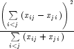
With this definition of variation, the Goodman and Kruskal
![]() coefficient for rows is computed as the reduction
of the total variation for rows accounted for by the columns, divided by the
total variation for the rows. To compute the reduction in the total
variation of the rows accounted for by the columns, note that the total
variation for the rows within column j is defined as follows:
coefficient for rows is computed as the reduction
of the total variation for rows accounted for by the columns, divided by the
total variation for the rows. To compute the reduction in the total
variation of the rows accounted for by the columns, note that the total
variation for the rows within column j is defined as follows:
![]()
The total variation for rows within columns is the sum of the
![]() variables. Consistent with the usual methods in the
analysis of variance, the reduction in the total variation is given as the
difference between the total variation for rows and the total variation for
rows within the columns.
variables. Consistent with the usual methods in the
analysis of variance, the reduction in the total variation is given as the
difference between the total variation for rows and the total variation for
rows within the columns.
Goodman and Kruskal's ![]() for columns is similarly
defined. See Bishop et al. (1975, p. 391) for the standard errors.
for columns is similarly
defined. See Bishop et al. (1975, p. 391) for the standard errors.
Uncertainty Coefficients: The uncertainty coefficient for rows is the increase in the log-likelihood that is achieved by the most general model over the independence model, divided by the marginal log-likelihood for the rows. This is given by the following equation:
The uncertainty coefficient for columns is similarly defined. The
symmetric uncertainty coefficient contains the same numerator as
![]() and
and ![]() but averages
the denominators of these two statistics. Standard errors for U are
given in Brown (1983).
but averages
the denominators of these two statistics. Standard errors for U are
given in Brown (1983).
Kruskal-Wallis: The Kruskal-Wallis statistic for rows is a one-way analysis-of-variance-type test that assumes the column variable is monotonically ordered. It tests the null hypothesis that no row populations are identical, using average ranks for the column variable. The Kruskal-Wallis statistic for columns is similarly defined. Conover (1980) discusses the Kruskal-Wallis test.
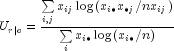
Test for Linear Trend: When there are two rows, it is possible to test for a linear trend in the row probabilities if it is assumed that the column variable is monotonically ordered. In this test, the probabilities for row 1 are predicted by the column index using weighted simple linear regression. This slope is given by
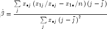
where
![]()
is the average column index. An asymptotic test that the slope is 0 may then be obtained (in large samples) as the usual regression test of zero slope.
In two-column data, a similar test for a linear trend in the column probabilities is computed. This test assumes that the rows are monotonically ordered.
Kappa: Kappa is a measure of agreement computed on square tables only. In the kappa statistic, the rows and columns correspond to the responses of two judges. The judges agree along the diagonal and disagree off the diagonal. Let
![]()
denote the probability that the two judges agree, and let
![]()
denote the expected probability of agreement under the independence
model. Kappa is then given by ![]() .
.
McNemar Tests: The McNemar test is a test of symmetry in a square
contingency table. In other words, it is a test of the null hypothesis
![]() . The multiple
degrees-of-freedom version of the McNemar test with
r (r - 1)/2 degrees of freedom is computed as follows:
. The multiple
degrees-of-freedom version of the McNemar test with
r (r - 1)/2 degrees of freedom is computed as follows:
![]()
The single degree-of-freedom test assumes that the differences,
![]() , are all in one direction. The single
degree-of-freedom test will be more powerful than the multiple
degrees-of-freedom test when this is the case. The test statistic is given
as follows:
, are all in one direction. The single
degree-of-freedom test will be more powerful than the multiple
degrees-of-freedom test when this is the case. The test statistic is given
as follows:
The exact probability can be computed by the binomial distribution.
| Constructor Summary | |
ContingencyTable(double[][] table)
Constructs and performs a chi-squared analysis of a two-way contingency table. |
|
| Method Summary | |
double |
getChiSquared()
Returns the Pearson chi-squared test statistic. |
double |
getContingencyCoef()
Returns contingency coefficient. |
double[][] |
getContributions()
Returns the contributions to chi-squared for each cell in the table. |
double |
getCramersV()
Returns Cramer's V. |
int |
getDegreesOfFreedom()
Returns the degrees of freedom for the chi-squared tests associated with the table. |
double |
getExactMean()
Returns exact mean. |
double |
getExactStdev()
Returns exact standard deviation. |
double[][] |
getExpectedValues()
Returns the expected values of each cell in the table. |
double |
getGSquared()
Returns the likelihood ratio G2 (chi-squared). |
double |
getGSquaredP()
Returns the probability of a larger G2 (chi-squared). |
double |
getP()
Returns the Pearson chi-squared p-value for independence of rows and columns. |
double |
getPhi()
Returns phi. |
double[][] |
getStatistics()
Returns the statistics associated with this table. |
| Methods inherited from class java.lang.Object |
clone, equals, finalize, getClass, hashCode, notify, notifyAll, toString, wait, wait, wait |
| Constructor Detail |
public ContingencyTable(double[][] table)
table - A double matrix containing the observed
counts in the contingency table.| Method Detail |
public double getChiSquared()
double scalar containing the Pearson
chi-squared test statistic.public double getContingencyCoef()
double scalar containing the contingency
coefficient based on Pearson chi-squared statistic.public double[][] getContributions()
double matrix of size (table.length+1) *
(table[0].length+1) containing the contributions
to chi-squared for each cell in the table. The last row and
column contain the total contribution to chi-squared for
that row or column.public double getCramersV()
double scalar containing the Cramer's V
based on Pearson chi-squared statistic.public int getDegreesOfFreedom()
int scalar containing the degrees of freedom
for the chi-squared tests associated with the table.public double getExactMean()
double scalar containing the exact mean
based on Pearson's chi-square statistic.public double getExactStdev()
double scalar containing the exact standard
deviation based on Pearson's chi-square statistic.public double[][] getExpectedValues()
double matrix of size (table.length+1) *
(table[0].length+1) containing the expected
values of each cell in the table, under the null hypothesis.
The marginal totals are in the last row and column.public double getGSquared()
double scalar containing the likelihood ratio
public double getGSquaredP()
double scalar containing the probability of
a larger public double getP()
double scalar containing the Pearson
chi-squared p-value for independence of rows and columns.public double getPhi()
double scalar containing the phi based on
Pearson chi-squared statistic.public double[][] getStatistics()
double matrix of size 23 * 5 containing
statistics associated with this table. Each row corresponds
to a statistic.
| Row | Statistics |
| 0 | gamma |
| 1 | Kendall's |
| 2 | Stuart's |
| 3 | Somers' D for rows (given columns) |
| 4 | Somers' D for columns (given rows) |
| 5 | product moment correlation |
| 6 | Spearman rank correlation |
| 7 | Goodman and Kruskal |
| 8 | Goodman and Kruskal |
| 9 | uncertainty coefficient U (symmetric) |
| 10 | uncertainty |
| 11 | uncertainty |
| 12 | optimal prediction |
| 13 | optimal prediction |
| 14 | optimal prediction |
| 15 | optimal prediction |
| 16 | optimal prediction |
| 17 | test for linear trend in row probabilities if
table.length = 2. If table.length is not 2, a test for linear trend
in column probabilities if table[0].length = 2. |
| 18 | Kruskal-Wallis test for no row effect |
| 19 | Kruskal-Wallis test for no column effect |
| 20 | kappa (square tables only) |
| 21 | McNemar test of symmetry (square tables only) |
| 22 | McNemar one degree of freedom test of symmetry (square tables only) |
If a statistic cannot be computed, or if some value is not relevant for the computed statistic, the entry is NaN (Not a Number).
The columns are as follows:
| Column | Value |
| 0 | estimated statistic |
| 1 | standard error for any parameter value |
| 2 | standard error under the null hypothesis |
| 3 | t value for testing the null hypothesis |
| 4 | p-value of the test in column 3 |
|
JMSLTM Numerical Library 4.0 | ||||||||
| PREV CLASS NEXT CLASS | FRAMES NO FRAMES | ||||||||
| SUMMARY: NESTED | FIELD | CONSTR | METHOD | DETAIL: FIELD | CONSTR | METHOD | ||||||||